#LLM

学习的所有代码都已经同步在 github 上，见Ecankk/Knowledge-Distillation

数据和模型

约 1510 个字 309 行代码 3 张图片 预计阅读时间 11 分钟

利用 CIFAR-10 数据集，用两个层次不一样的模型作为教师模型和学生模型

Python

# Deeper neural network class to be used as teacher:
class DeepNN(nn.Module):
    def __init__(self, num_classes=10):
        super(DeepNN, self).__init__()
        self.features = nn.Sequential(
            nn.Conv2d(3, 128, kernel_size=3, padding=1),
            nn.ReLU(),
            nn.Conv2d(128, 64, kernel_size=3, padding=1),
            nn.ReLU(),
            nn.MaxPool2d(kernel_size=2, stride=2),
            nn.Conv2d(64, 64, kernel_size=3, padding=1),
            nn.ReLU(),
            nn.Conv2d(64, 32, kernel_size=3, padding=1),
            nn.ReLU(),
            nn.MaxPool2d(kernel_size=2, stride=2),
        )
        self.classifier = nn.Sequential(
            nn.Linear(2048, 512),
            nn.ReLU(),
            nn.Dropout(0.1),
            nn.Linear(512, num_classes)
        )

    def forward(self, x):
        x = self.features(x)
        x = torch.flatten(x, 1)
        x = self.classifier(x)
        return x

# Lightweight neural network class to be used as student:
class LightNN(nn.Module):
    def __init__(self, num_classes=10):
        super(LightNN, self).__init__()
        self.features = nn.Sequential(
            nn.Conv2d(3, 16, kernel_size=3, padding=1),
            nn.ReLU(),
            nn.MaxPool2d(kernel_size=2, stride=2),
            nn.Conv2d(16, 16, kernel_size=3, padding=1),
            nn.ReLU(),
            nn.MaxPool2d(kernel_size=2, stride=2),
        )
        self.classifier = nn.Sequential(
            nn.Linear(1024, 256),
            nn.ReLU(),
            nn.Dropout(0.1),
            nn.Linear(256, num_classes)
        )

    def forward(self, x):
        x = self.features(x)
        x = torch.flatten(x, 1)
        x = self.classifier(x)
        return x

初次蒸馏尝试

直接尝试在分类的结果上对齐

蒸馏函数（针对结果的对齐）

Python

def train_knowledge_distillation(teacher, student, train_loader, epochs, learning_rate, T, soft_target_loss_weight, ce_loss_weight, device):
    ce_loss = nn.CrossEntropyLoss()
    optimizer = optim.Adam(student.parameters(), lr=learning_rate)

    teacher.eval()  # Teacher set to evaluation mode
    student.train() # Student to train mode

    for epoch in range(epochs):
        running_loss = 0.0
        for inputs, labels in train_loader:
            inputs, labels = inputs.to(device), labels.to(device)

            optimizer.zero_grad()

            # Forward pass with the teacher model - do not save gradients here as we do not change the teacher's weights
            with torch.no_grad():
                teacher_logits = teacher(inputs)

            # Forward pass with the student model
            student_logits = student(inputs)

            #Soften the student logits by applying softmax first and log() second
            soft_targets = nn.functional.softmax(teacher_logits / T, dim=-1)
            soft_prob = nn.functional.log_softmax(student_logits / T, dim=-1)

            # Calculate the soft targets loss. Scaled by T**2 as suggested by the authors of the paper "Distilling the knowledge in a neural network"
            soft_targets_loss = torch.sum(soft_targets * (soft_targets.log() - soft_prob)) / soft_prob.size()[0] * (T**2)

            # Calculate the true label loss
            label_loss = ce_loss(student_logits, labels)

            # Weighted sum of the two losses
            loss = soft_target_loss_weight * soft_targets_loss + ce_loss_weight * label_loss

            loss.backward()
            optimizer.step()

            running_loss += loss.item()

        print(f"Epoch {epoch+1}/{epochs}, Loss: {running_loss / len(train_loader)}")

- teacher：预训练的教师模型（如 DeepNN）。
- student：待训练的学生模型（如 LightNN）。
- train_loader：训练数据加载器，提供输入和标签。
- epochs：训练轮数。
- learning_rate：优化器学习率。
- T：温度参数，用于软化概率分布。
- soft_target_loss_weight：蒸馏损失的权重。
- ce_loss_weight：交叉熵损失的权重。
- device：运行设备

T 对蒸馏的影响

软化：通过增大 T ，减少 logits 的相对差异，使概率分布更均匀。
利用 T 软化 softmax 的概率分布，让输出更倾向于分布而不是分类本身

\[ p(i) = \frac{\exp(z_i / T)}{\sum_j \exp(z_j / T)} \]

从而区别于数据集给出的这个图象是什么，而是让教师模型告诉学生模型，这张图很像 a，但也有一点像 b

T 越大，分布越平滑，次要类别概率越高。

蒸馏损失公式

\[ \text{soft\_targets\_loss} = \frac{\sum \left( p_{teacher} \cdot (\log p_{teacher} - \log p_{student}) \right)}{\text{batch\_size}} \cdot T^2 \]

• \(T^2\) 补偿梯度减小，确保损失对优化的贡献稳定
• 此处的蒸馏损失是 KL 散度的变体，用于衡量两个概率分布的差异

蒸馏结果 1

Text Only

Teacher accuracy: 75.49%
Student accuracy without teacher: 70.81%
Student accuracy with CE + KD: 71.40%

感觉有提升，但是提升不大，感觉老师本身就不够优秀

CosineEmbeddingLoss

• 余弦相似度

\[ \text{cosine\_similarity}(x_1, x_2) = \cos(\theta) = \frac{x_1 \cdot x_2}{\|x_1\| \|x_2\|} \]

• 损失定义

\[ \text{loss}(x_1, x_2, y) = \begin{cases} 1 - \cos(x_1, x_2), & \text{if } y = 1 \\ \max(0, \cos(x_1, x_2) - \text{margin}), & \text{if } y = -1 \end{cases} \]

1. 对于正样本 y=1
   1. 让两个向量尽肯能的对齐，如果完全对齐的话 \(cos(x_1,x_2)\) 为 1，损失为 0
2. 对于负样本 y=-1
   1. 使 \(cos(x_1,x_2)\) 小于 margin，即让 \(x_1\) 和 \(x_2\) 尽可能不相似
3. Margin 的作用
   1. 定义边界：负样本对的相似度低于 margin \text{margin} margin 时无需惩罚。
   2. 选择：
      • margin=0：严格要求负样本正交。
      • margin=0.5：允许一定相似度，增加鲁棒性。

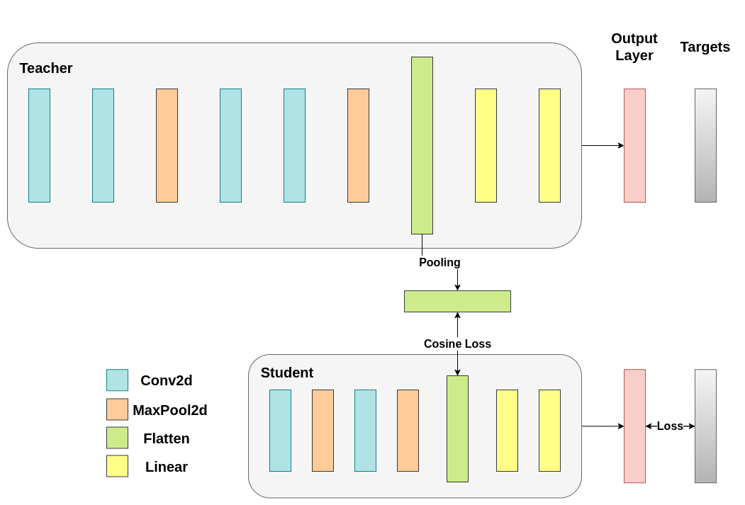
第一次修改模型

在之前的模型中，我们知识讲蒸馏损失应用于输出层 logits，此时两者的输出维度是相同的，都是十种分类的输出，但是我们希望学生模型能够学习教师模型的 flattened convolutional output 即卷积层（特征提取器）的输出和全连接层（分类器）的输入，但是这样就有了一个新的问题，两者的尾部不符合，教室是 2048 而学生是 1024. 这个时候就需要修改模型了

Python

class ModifiedDeepNNCosine(nn.Module):
    def __init__(self, num_classes=10):
        super(ModifiedDeepNNCosine, self).__init__()
        self.features = nn.Sequential(
            nn.Conv2d(3, 128, kernel_size=3, padding=1),
            nn.ReLU(),
            nn.Conv2d(128, 64, kernel_size=3, padding=1),
            nn.ReLU(),
            nn.MaxPool2d(kernel_size=2, stride=2),
            nn.Conv2d(64, 64, kernel_size=3, padding=1),
            nn.ReLU(),
            nn.Conv2d(64, 32, kernel_size=3, padding=1),
            nn.ReLU(),
            nn.MaxPool2d(kernel_size=2, stride=2),
        )
        self.classifier = nn.Sequential(
            nn.Linear(2048, 512),
            nn.ReLU(),
            nn.Dropout(0.1),
            nn.Linear(512, num_classes)
        )

    def forward(self, x):
        x = self.features(x)  # 卷积输出：[batch_size, 32, 8, 8]
        flattened_conv_output = torch.flatten(x, 1)  # 展平：[batch_size, 2048]
        x = self.classifier(flattened_conv_output)  # 分类器输出：[batch_size, 10]
        flattened_conv_output_after_pooling = torch.nn.functional.avg_pool1d(flattened_conv_output, 2)  # 池化：[batch_size, 1024]
        return x, flattened_conv_output_after_pooling  # 返回元组

class ModifiedLightNNCosine(nn.Module):
    def __init__(self, num_classes=10):
        super(ModifiedLightNNCosine, self).__init__()
        self.features = nn.Sequential(
            nn.Conv2d(3, 16, kernel_size=3, padding=1),
            nn.ReLU(),
            nn.MaxPool2d(kernel_size=2, stride=2),
            nn.Conv2d(16, 16, kernel_size=3, padding=1),
            nn.ReLU(),
            nn.MaxPool2d(kernel_size=2, stride=2),
        )
        self.classifier = nn.Sequential(
            nn.Linear(1024, 256),
            nn.ReLU(),
            nn.Dropout(0.1),
            nn.Linear(256, num_classes)
        )

    def forward(self, x):
        x = self.features(x)  # 卷积输出：[batch_size, 16, 8, 8]
        flattened_conv_output = torch.flatten(x, 1)  # 展平：[batch_size, 1024]
        x = self.classifier(flattened_conv_output)  # 分类器输出：[batch_size, 10]
        return x, flattened_conv_output  # 返回元组

* 变动就是对教师模型的 feature 层的输出进行了一次平均池化，让 2048 压缩为 1024，从而能够指导学生模型
* 模型的输出除了分类的结果，再返回一个展平后的卷积层(feature层) 的输出

修改蒸馏函数

Python

def train_cosine_loss(teacher, student, train_loader, epochs, learning_rate, hidden_rep_loss_weight, ce_loss_weight, device):
    ce_loss = nn.CrossEntropyLoss()
    cosine_loss = nn.CosineEmbeddingLoss()
    optimizer = optim.Adam(student.parameters(), lr=learning_rate)

    teacher.to(device)
    student.to(device)
    teacher.eval()  # Teacher set to evaluation mode
    student.train() # Student to train mode

    for epoch in range(epochs):
        running_loss = 0.0
        for inputs, labels in train_loader:
            inputs, labels = inputs.to(device), labels.to(device)

            optimizer.zero_grad()

            # Forward pass with the teacher model and keep only the hidden representation
            with torch.no_grad():
                _, teacher_hidden_representation = teacher(inputs)

            # Forward pass with the student model
            student_logits, student_hidden_representation = student(inputs)

            # Calculate the cosine loss. Target is a vector of ones. From the loss formula above we can see that is the case where loss minimization leads to cosine similarity increase.
            hidden_rep_loss = cosine_loss(student_hidden_representation, teacher_hidden_representation, target=torch.ones(inputs.size(0)).to(device))

            # Calculate the true label loss
            label_loss = ce_loss(student_logits, labels)

            # Weighted sum of the two losses
            loss = hidden_rep_loss_weight * hidden_rep_loss + ce_loss_weight * label_loss

            loss.backward()
            optimizer.step()

            running_loss += loss.item()

        print(f"Epoch {epoch+1}/{epochs}, Loss: {running_loss / len(train_loader)}")

def test_multiple_outputs(model, test_loader, device):
    model.to(device)
    model.eval()

    correct = 0
    total = 0

    with torch.no_grad():
        for inputs, labels in test_loader:
            inputs, labels = inputs.to(device), labels.to(device)

            outputs, _ = model(inputs) # Disregard the second tensor of the tuple
            _, predicted = torch.max(outputs.data, 1)

            total += labels.size(0)
            correct += (predicted == labels).sum().item()

    accuracy = 100 * correct / total
    print(f"Test Accuracy: {accuracy:.2f}%")
    return accuracy

蒸馏结果

Test Accuracy: 70.69% 感觉更不行，高维向量更难以提取有意义的特征，盲目追求向量的匹配并不能带来

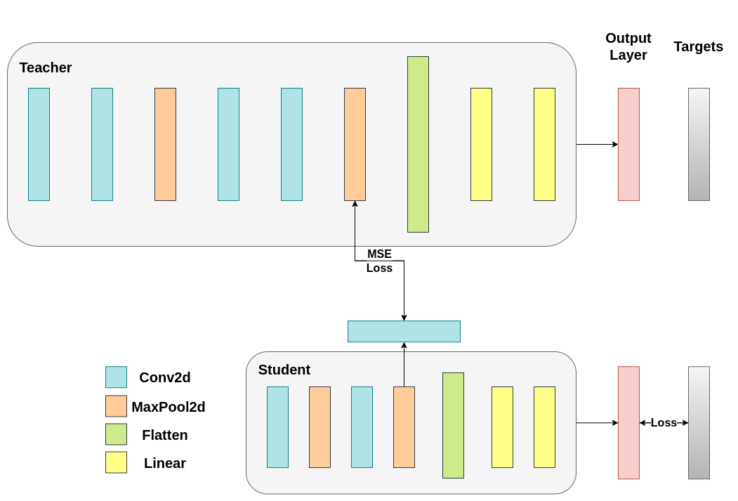
第二次修改

放弃直接匹配展平向量，改为匹配卷积层输出的特征图

特征图的生成过程

• 卷积核（Filter/Kernel）：
  • 一个小的权重矩阵（如 [3, 3]），用于检测输入中的特定模式（如边缘、纹理）。
  • 每个卷积核生成一个特征图通道。
• 计算：
  • 卷积核在输入上滑动（卷积运算），每次计算局部区域的加权和，生成一个值。
  • 滑动完成后，形成一个二维特征图。
• 公式

\[ \text{Feature Map}_{i,j} = \sum_{m,n} \text{Input}_{i+m, j+n} \cdot \text{Kernel}_{m,n} + \text{Bias} \]

因此，一次卷积操作（用一个卷积核扫一遍图像），输出就是一张特征图，他代表神经网络在某一方面提取到的某个特征

查看特征图的尺寸

Text Only

Student's feature extractor output shape:  torch.Size([128, 16, 8, 8])
Teacher's feature extractor output shape:  torch.Size([128, 32, 8, 8])

这意味着教室模型用了 32 个卷积核，有 32 张特征图，而学生只有 16 张，接下来需要讲学生的特征图转换成教师的特征图的形状

修改的目的

我们希望额外添加一个欸外的中间层来把学生模型的 16 层特征图转换为 32 层特征图，也就是额外增加一个卷积层把通道从 16 转换成 32。

修改后的模型

Python

class ModifiedDeepNNRegressor(nn.Module):
    def __init__(self, num_classes=10):
        super(ModifiedDeepNNRegressor, self).__init__()
        self.features = nn.Sequential(
            nn.Conv2d(3, 128, kernel_size=3, padding=1),
            nn.ReLU(),
            nn.Conv2d(128, 64, kernel_size=3, padding=1),
            nn.ReLU(),
            nn.MaxPool2d(kernel_size=2, stride=2),
            nn.Conv2d(64, 64, kernel_size=3, padding=1),
            nn.ReLU(),
            nn.Conv2d(64, 32, kernel_size=3, padding=1),
            nn.ReLU(),
            nn.MaxPool2d(kernel_size=2, stride=2),
        )
        self.classifier = nn.Sequential(
            nn.Linear(2048, 512),
            nn.ReLU(),
            nn.Dropout(0.1),
            nn.Linear(512, num_classes)
        )

    def forward(self, x):
        x = self.features(x)
        conv_feature_map = x
        x = torch.flatten(x, 1)
        x = self.classifier(x)
        return x, conv_feature_map

class ModifiedLightNNRegressor(nn.Module):
    def __init__(self, num_classes=10):
        super(ModifiedLightNNRegressor, self).__init__()
        self.features = nn.Sequential(
            nn.Conv2d(3, 16, kernel_size=3, padding=1),
            nn.ReLU(),
            nn.MaxPool2d(kernel_size=2, stride=2),
            nn.Conv2d(16, 16, kernel_size=3, padding=1),
            nn.ReLU(),
            nn.MaxPool2d(kernel_size=2, stride=2),
        )
        # Include an extra regressor (in our case linear)
        self.regressor = nn.Sequential(
            nn.Conv2d(16, 32, kernel_size=3, padding=1)
        )
        self.classifier = nn.Sequential(
            nn.Linear(1024, 256),
            nn.ReLU(),
            nn.Dropout(0.1),
            nn.Linear(256, num_classes)
        )

    def forward(self, x):
        x = self.features(x)
        regressor_output = self.regressor(x)
        x = torch.flatten(x, 1)
        x = self.classifier(x)
        return x, regressor_output

取消了对卷积层的展平，直接输出特征图，为学生模型添加了一个新的卷积层用于特征图类型的匹配

训练步骤的修改

主要是针对特征图的损失，因为两者的形状相同，利用均方误差可以衡量，只需要修改训练的函数就行了

Python

def train_mse_loss(teacher, student, train_loader, epochs, learning_rate, feature_map_weight, ce_loss_weight, device):
    ce_loss = nn.CrossEntropyLoss()
    mse_loss = nn.MSELoss()
    optimizer = optim.Adam(student.parameters(), lr=learning_rate)

    teacher.to(device)
    student.to(device)
    teacher.eval()  # Teacher set to evaluation mode
    student.train() # Student to train mode

    for epoch in range(epochs):
        running_loss = 0.0
        for inputs, labels in train_loader:
            inputs, labels = inputs.to(device), labels.to(device)

            optimizer.zero_grad()

            # Again ignore teacher logits
            with torch.no_grad():
                _, teacher_feature_map = teacher(inputs)

            # Forward pass with the student model
            student_logits, regressor_feature_map = student(inputs)

            # Calculate the loss
            hidden_rep_loss = mse_loss(regressor_feature_map, teacher_feature_map)

            # Calculate the true label loss
            label_loss = ce_loss(student_logits, labels)

            # Weighted sum of the two losses
            loss = feature_map_weight * hidden_rep_loss + ce_loss_weight * label_loss

            loss.backward()
            optimizer.step()

            running_loss += loss.item()

        print(f"Epoch {epoch+1}/{epochs}, Loss: {running_loss / len(train_loader)}")

训练结果

Test Accuracy: 71.13% 比之展平后使用 CosineLoss 的结果好，但是不如第一种直接根据结果训练，不过差距很小了

结果汇总

Text Only

Teacher accuracy: 75.49%
Student accuracy without teacher: 70.81%
Student accuracy with CE + KD: 71.40%
Student accuracy with CE + CosineLoss: 70.69%
Student accuracy with CE + RegressorMSE: 71.13%

模型蒸馏的意义

我们并没有添加额外的参数，因此蒸馏后的模型的推理时间并没有增加，开销仅仅是在重新训练学生模型时候的梯度计算的开销。因此模型蒸馏史很有意义的，这里仅仅是简单的尝试，因该会有更多有意的方法和参数调整让模型的学习更有意义，比如同时加上 KD 和 RegressorMSE？（尝试了一下效果更不好，一味的模仿估计是不行的）

参考资料

知识蒸馏教程 — PyTorch 教程 2.6.0+cu124 文档 --- Knowledge Distillation Tutorial — PyTorch Tutorials 2.6.0+cu124 documentation
[1503.02531] Distilling the Knowledge in a Neural Network

Knowledge Distillation Tutorial — PyTorch Tutorials 2.6.0+cu124 documentation